 Bookmarks: Bookmarks:
Links Terms
Tools
6s & the Org
6s Define
6s Measure 6s Analyze
6s Improve and Control References
|
|
|
- Terms
- A CTQ tree (Critical-to-quality tree) is used to decompose broad customer requirements into more easily quantified requirements. CTQ Trees are often used in the Six Sigma methodology (Wikipedia, 2010).
- Common-and special-causes are the two distinct origins of variation in a process, as defined in the statistical thinking and methods of Walter A. Shewhart and W. Edwards Deming. Briefly, “common-cause” is the usual, historical, quantifiable variation in a system, while “special-causes” are unusual, not previously observed, non-quantifiable variation (Wikipedia, 2010).
- Six Sigma projects follow two project methodologies inspired by Deming’s Plan-Do-Check-Act Cycle. The PDCA cycle consists of four steps: Plan, Do, Check, and Act. PDCA is a logical representation of how people naturally approach problems. The “Classical approach”, “PDCA”, and “PDSA” methodologies make use of the seven original quality tools and do not typically require a statistical approach. The seven original quality tools are as follows (Skillsoft, 2010):These methodologies, composed of five phases each, bear the acronyms DMAIC and DMADV (Wikipedia, 2010).
- During the Plan step of the PDCA cycle, the plan for improvement is created. The plan is not enacted until the Do step.
- The second step of the PDCA cycle, Do, is when the
plan for improvement, created in the Plan step, is implemented.
- During the Check step of the PDCA cycle, the results of the implemented plan from the Do step are measured and analyzed.
- During the Act step of the PDCA cycle, if results from the Check step differ from the expected outcome, changes and reforms to the process are made.
- Check sheets
- Pareto diagrams
- Process flow diagrams
- Scatter diagrams
- Run charts
- Histograms
- Fishbone diagrams
- DMAIC
- Define the problem, the voice of the customer, and the project goals, specifically. Choose an appropriate target for the Six Sigma initiative.
- Measure key aspects of the current process and collect relevant data. Gather data on the target to be improved.
- Analyze the data to investigate and verify cause-and-effect relationships. Determine what the relationships are, and attempt to ensure that all factors have been considered. Seek out root cause of the defect under investigation. Identify the root causes of defects or deviations in the target.
- Improve or optimize the current process based upon data analysis using techniques such as design of experiments, poka yoke or mistake proofing, and standard work to create a new, future state process. Set up pilot runs to establish process capability. Implement a change to eliminate the cause of defects or deviations in the target.
- Control the future state process to ensure that any deviations from target are corrected before they result in defects. Control systems are implemented such as statistical process control, production boards, and visual workplaces and the process is continuously monitored. Monitor the newly implemented process to ensure that improvements last.
- The Define, Measure, Analyze, Improve, Control (DMAIC) process is a cyclical process that makes use of many statistical techniques. The DMAIC methodology typically requires professionals trained in the use of statistical software. Some statistics-oriented techniques used by DMAIC include the following:
- Quality Function Deployment (QFD)
- Failure modes and effects analysis (FMEA)
- Process capability
- Multi-vari analysis
- Analysis of variance (ANOVA)
- Regression analysis
- Design of Experiments (DoE)
- Hypothesis testing
- Control plans
- Measurement system analysis
- Mistake proofing
- Confidence intervals
- DMADV project methodology, also known as DFSS (“Design For Six Sigma”), features five phases:
- Define design goals that are consistent with customer demands and the enterprise strategy.
- Measure and identify CTQs (characteristics that are Critical To Quality), product capabilities, production process capability, and risks.
- Analyze to develop and design alternatives, create a high-level design and evaluate design capability to select the best design.
- Design details, optimize the design, and plan for design verification. This phase may require simulations.
- Verify the design, set up pilot runs, implement the production process and hand it over to the process owner(s).
- DFSS is distinctly different from classic Six Sigma. Whereas classic Six Sigma is a methodology focused on the optimization of the manufacturing process, DFSS is a newer method that encompasses the entire product development cycle. This necessarily includes the front end product definition, design, and ideation activities. While DFSS does not formally include specific tools for innovation, the DFSS process does contain a natural insertion point for innovation best practices to fill the innovate-here step.
|
Links
Terms
Tools
6s & the Org
6s Define
6s Measure 6s Analyze
6s Improve and Control References |
- Tools
- Quality Function Deployment (QFD): The QFD is used to understand customer requirements. The “deployment” part comes from the fact that quality engineers used to be deployed to customer locations to fully understand a customer’s needs. Today, a physical deployment might not take place, but the idea behind the tool is still valid. Basically, the QFD identifies customer requirements and rates them on a numerical scale, with higher numbers corresponding to pressing “must-haves” and lower numbers to “nice-to-haves.” Then, various design options are listed and rated on their ability to address the customer’s needs. Each design option earns a score, and those with high scores become the preferred solutions to pursue (How Stuff Works, 2010).
- Fishbone Diagrams: In Six Sigma, all outcomes are the result of specific inputs. This cause-and-effect relationship can be clarified using either a fishbone diagram or a cause-and-effect matrix (see below). The fishbone diagram helps identify which input variables should be studied further. The finished diagram looks like a fish skeleton, which is how it earned its name. To create a fishbone diagram, you start with the problem of interest — the head of the fish. Then you draw in the spine and, coming off the spine, six bones on which to list input variables that affect the problem. Each bone is reserved for a specific category of input variable, as shown below. After listing all input variables in their respective categories, a team of experts analyzes the diagram and identifies two or three input variables that are likely to be the source of the problem (How Stuff Works, 2010).
- Cause-and-Effect (C&E) Matrix: The C&E matrix is an extension of the fishbone diagram. It helps Six Sigma teams identify, explore and graphically display all the possible causes related to a problem and search for the root cause. The C&E Matrix is typically used in the Measure phase of the DMAIC methodology (How Stuff Works, 2010).
- T-Test: In Six Sigma, you need to be able to establish a confidence level about your measurements. Generally, a larger sample size is desirable when running any test, but sometimes it’s not possible. The T-Test helps Six Sigma teams validate test results using sample sizes that range from two to 30 data points (How Stuff Works, 2010).
- Control Charts: Statistical process control, or SPC, relies on statistical techniques to monitor and control the variation in processes. The control chart is the primary tool of SPC. Six Sigma teams use control charts to plot the performance of a process on one axis versus time on the other axis. The result is a visual representation of the process with three key components: a center line, an upper control limit and a lower control limit. Control charts are used to monitor variation in a process and determine if the variation falls within normal limits or is variation resulting from a problem or fundamental change in the process (How Stuff Works, 2010).
- Design of Experiments: When a process is optimized, all inputs are set to deliver the best and most stable output. The trick, of course, is determining what those input settings should be. A design of experiments, or DOE, can help identify the optimum input settings. Performing a DOE can be time-consuming, but the payoffs can be significant. The biggest reward is the insight gained into the process (How Stuff Works, 2010).
- Null Hypothesis – The null hypothesis can be rejected or failed to be rejected. For example, if you want to test the difference of two means and determine they are different, then the null hypothesis that states they are the same is rejected (Skillsoft, 2010).
- Mutually Exclusive – events can be defined as two events, A and B, which have no answer points in common. The probability of mutually exclusive events occurring at the same time is 0 (Skillsoft, 2010).
- Gage Technique – Control plans display information in lines. Each line consists of multiple items. The gage technique, also known as the measurement technique, is an example of a line item that describes how measurements are made. e.g. measurement of length would contain steel ruler.
- Win-Win Negotiations Philosophy
- Create Win-Win Plans
- Build Win-Win Relationships
- Engineer Win-Win Agreements
- Carry out Win-Win Maintenance
- In a Lean Production system the Takt Time is the time interval between consecutive items in a production system that must be achieved to to meet customer demand. If the daily customer demand is 40 items and there are 400 minutes of production time then the takt time is 10 minutes. The takt time is the ‘heartbeat’ for a Just In Time production system (‘takt’ is the German word for a conductor’s baton). The idea is that production should be paced to produce one item every ten minutes rather than in periodic batches (MiC Quality, 2010).
- Residuals are the differences between observed values and the corresponding values predicted by a model. e.g. In regression analysis, once you come up with a line that fits the data, you can determine how well the line fits by looking at the residuals.
- UCL = X-double bar + (A2 * R-Bar)
- LCL = X-double bar – (A2 * R-Bar)
- Table of Control Chart Constants
- Control charts (Engineering Statistics Handbook, 2010)
- Control charts dealing with the number of defects or nonconformities are called c charts (for count)
- Control charts dealing with the proportion or fraction of defective product are called p charts (for proportion).
- Defects per unit, is called the u chart (for unit). This applies when we wish to work with the average number of nonconformities per unit of product.
- Tuckman’s Group Development Model – The Forming – Storming – Norming – Performing is a model of group development, first proposed by Bruce Tuckman in 1965, who maintained that these phases are all necessary and inevitable in order for the team to grow, to face up to challenges, to tackle problems, to find solutions, to plan work, and to deliver results. This model has become the basis for subsequent models (Wikipedia, 2010).
- Forming – In the first stages of team building, the forming of the team takes place. The individual’s behavior is driven by a desire to be accepted by the others, and avoid controversy or conflict.
- Storming – Every group will then enter the storming stage in which different ideas compete for consideration. The team addresses issues such as what problems they are really supposed to solve, how they will function independently and together and what leadership model they will accept. Team members open up to each other and confront each other’s ideas and perspectives.
- Norming – The team manages to have one goal and come to a mutual plan for the team at this stage. Some may have to give up their own ideas and agree with others in order to make the team work.
- Performing – It is possible for some teams to reach the performing stage. These high-performing teams are able to function as a unit as they find ways to get the job done smoothly and effectively without inappropriate conflict or the need for external supervision. Team members have become interdependent. By this time they are motivated and knowledgeable. The team members are now competent, autonomous and able to handle the decision-making process without supervision.
- The Deming-Shewhart cycle is also known as the Plan, Do, Study, Act (PDSA) project methodology. The effects of a change or test that is enacted in the Do step of the cycle are observed, recorded, and analyzed in the Study step. During the Plan step of the PDSA cycle, desirable changes. required data. and a test plan are agreed upon by the project team. During the Do step of the PDSA cycle. the test or changes agreed upon in the Plan
- Statistical process control (SPC) charts are used as a form of quality control. They are deployed during process baseline estimation to monitor the variables and parameters occurring within a particular process. The performance of these variables is tracked in relation to predetermined upper and lower control limits (Skillsoft, 2010).
|
|
- 6s & the Organization
- Key Roles (Wikipedia, 2010):
- Executive Leadership includes the CEO and other members of top management. They are responsible for setting up a vision for Six Sigma implementation. They also empower the other role holders with the freedom and resources to explore new ideas for breakthrough improvements.
- Champions take responsibility for Six Sigma implementation across the organization in an integrated manner. The Executive Leadership draws them from upper management.
- Master Black Belts, identified by champions, act as in-house coaches on Six Sigma. They devote 100% of their time to Six Sigma. They assist champions and guide Black Belts and Green Belts. Apart from statistical tasks, they spend their time on ensuring consistent application of Six Sigma across various functions and departments.
- Black Belts operate under Master Black Belts to apply Six Sigma methodology to specific projects. They devote 100% of their time to Six Sigma. They primarily focus on Six Sigma project execution, whereas Champions and Master Black Belts focus on identifying projects/functions for Six Sigma.
- Green Belts, the employees who take up Six Sigma implementation along with their other job responsibilities, operate under the guidance of Black Belts.
- Yellow Belts, trained in the basic application of Six Sigma management tools, work with the Black Belt throughout the project stages and are often the closest to the work.
- Muda
- Waiting muda occurs whenever an operator is unable to work, even though they are ready and able. This can occur due to machine downtime, lack of parts, unwarranted monitoring activities, or line stoppages.
- Motion muda occurs when a process requires inefficient use of human motion. Examples of motion muda include excessive walking, heavy lifting, bending awkwardly, overreaching, and repetitive motion.
- Processing muda occurs when extra steps in the manufacturing process do not add value to the product for the consumer. Examples of processing muda include removing burrs from a manufacturing process. reshaping an item due to poor dies, and performing product inspections.
- Transport muda occurs whenever an item is moved. All forms of transportation are considered non-value—added actions. Reducing the number of times an item must be moved, or reducing the distance it must be moved. will reduce transport muda.
- Value Stream Maps visually depicts all activities involved in product manufacturing.
- Circle with a smile – Operator
- Three Peaked Roof – Supplier
- Upside Down Triangle – Kanban signal
- Right Side Up Triangle with I – Inventory
- Quality Pioneers
- Cycle time is the amount of time it takes to complete a single operation in the manufacturing process. Takt time refers to the amount of time it takes to complete a single product. When the cycle time of all operations in a process is equal to the takt time, single-piece-flow is achieved. Single-piece flow occurs when a product proceeds through each operation in manufacturing without interruption, back-flow, or scrap. This will eliminate waste in the process, as items never have to wait between operations.
- Failure Modes and Effects Analysis (FMEA): FMEA combats Murphy’s Law by identifying ways a new product, process or service might fail. FMEA isn’t worried just about issues with the Six Sigma project itself, but with other activities and processes that are related to the project. It’s similar to the QFD in how it is set up. First, a list of possible failure scenarios is listed and rated by importance. Then a list of solutions is presented and ranked by how well they address the concerns. This generates scores that enable the team to prioritize things that could go wrong and develop preventative measures targeted at the failure scenarios (How Stuff Works, 2010). Failure Mode and Effects Analysis (FMEA) is designed to decrease or, ideally, eliminate the number of failures or errors in a product or process. The four common types of FMEAs are system, design, process, and service. Regardless of type, the high-level steps for FMEA are as follows (Skillsoft, 2010):
- Choose a process to analyze
- Observe the process
- Make note of potential failure modes
- Rate potential failure modes for severity, occurrences. and detection levels
- Based on the previous ratings, calculate the risk priority number (RPN)
- Take actions to correct the failure modes with the highest RPNs and recalculate RPNs
- Update the table of observed failure modes
Performing a failure modes and effects analysis (FMEA) will assist in Ending the next target for improvement based on criticality of failure modes. An FMEA identities issues and their probability of occurrence, severity, and the effectiveness of control measures currently in place to catch the issue. An index of these values is created for each issue. To determine which issue needs to be assessed next. a risk priority number (RPN) must be calculated. RPN is calculated by multiplying the values of the previously generated indices. The issue with the highest RPN, or the issue with the highest severity, would then be the next to be addressed.
- There are typically eight steps performed when developing a balanced scorecard:
- Step 1; The scope of the card is defined.
- Step 2: A facilitator gathers information from senior management for the scorecard.
- Step 3; The facilitator presents the gathered information at an executive workshop to develop a draft of the scorecard’s measures.
- Step 4: The facilitator creates a rough draft of the scorecard and a new report.
- Step 5: A second executive workshop is held to refine the drafted scorecard and objectives for the measures are defined.
- Step 6: A third workshop is conducted to finalize the vision, objectives, and measures.
- Step 7; A task team develops an implementation plan.
- Step 8: The balanced scorecard is periodically reviewed.
- Failure Mode and Effects Analysis (FMEA)
- Process FMEAs (PFNlEAs) are concerned with manufacturing and assembly processes. PFMEAs examine and attempt to minimize the causes of failures by operations performed in the manufacturing and assembly process. A PFMEA is typically done before or alter the feasibility stage of development and prior to the tooling of machines used in the manufacturing process.
- System FMEAs (SFMEAS) are done with systems, subsystems, components, and their interactions.
- Design FMEAs (DFMEAs) deal with failures modes relating to design deficiencies in the product.
- Service FMEAs deal with services provided to the customer.
- There are three basic measures used in evaluating systems using the Theory of Constraints (TOC): throughput, inventory, and operational expenses. Throughput is how fast a system generates money through sales. Inventory refers to all money spent on things that will be sold. Operational expenses refer to expenditures made to turn inventory into throughput. While machine efficiency, equipment utilization, and downtime can be measures used in evaluating a system, they are not considered basic measures. Applying the TOC is a live-step method. The live steps are described as follows:
- Step 1 – Identify the system’s constraints.
- Step 2 – Decide how to exploit the system’s constraints.
- Step 3 – Subordinate everything else to the above decisions.
- Step 4 – Elevate the system’s constraints.
- Step 5 – Return to Step 1.
- Automating a process is good way of reducing defects due to human error. Automating a poorly designed process, however, may not have the desired effect. It may decrease defect levels, but it is just as likely to result in the stabilization of defect levels. A process should be well designed and stabilized before it is considered for automation.
- Organizations new to the Six Sigma philosophy will typically progress through the following
sequence of events:
- Training and launch: The organization learns about the Define, Measure, Analyze, Improve, and Control (DMAIC) approach to problem solving, and projects for obvious improvement opportunities are initiated.
- Implementation: Core business objectives are the target of improvement projects. A more statistically intensive approach is applied to all improvement projects.
- DFSS: As the organization becomes more comfortable with Six Sigma objectives, the undertaking of complex projects with a higher potential for gains increases and new products are designed with Six Sigma efficiency in mind.
- Just-in-time (JIT) refers to the concept that items are produced and delivered at exactly the right time and in exactly the right amount. JIT is related to the concept of single-piece flow where a single item flows through each stage of a process without delay.
- The concept of level loading involves balancing a process’s throughput over time.
- Perfection is the elimination of all waste (muda) from a process.
|
|
- 6s Define
- A focus group will produce a greater number of comments than individual interviews. This is due to members of the group stimulating each other’s responses. The group’s interviewer is able to direct conversation with probing questions to clarify the group’s comments. The results from a focus group are expressed in the participant’s own words, which lend to high face validity. Some disadvantages of a focus group are:
- dialogue is sometimes difficult to analyze due to multiple interactions between the participants.
- results often depend on the skill of the group’s interviewer. Skilled focus group interviewers are difficult to find.
- a loss of control compared to individual interviews. Although an interviewer may direct some of the dialogue of a focus group, the interaction of the group’s participants reduces the interviewers control.
- Consequential metrics are also known as secondary metrics and are derived from the primary metrics. Examples of consequential metrics include defects per unit (DPU), defects per million opportunities (DPMO), average age of receivables, lines of error free software code, and reduction in scrap. Cycle time, labor, and cost are examples of primary, also known as basic, metrics.
- Project Closure
- During the postmortem analysis project closure step, a committee of qualified company personnel will formally review and critique a project. This step is also known as lessons learned, autopsy, or post-project appraisal. The scope of the review extends over all phases of the project’s lifecycle from beginning to end. Examples of topics covered by the postmortem analysis include the following:
- Were adequate personnel, time. equipment. and money devoted to the project?
- Was the project effective?
- How well was the project tracked?
- Was the project sponsor and top management properly informed of the project’s status throughout the project’s lifecycle?
- How well did the project team work together?
- Were the project team’s efforts sufficiently recognized?
- How effective were corrective actions throughout the project’s lifecycle?
- What is the quality level of the delivered product or service?
- The final report step of the project is an evaluation of the project’s performance. It documents the completion of objectives and compares the project’s costs and realized benefits. The final report also documents a comparison between actual activity completion dates and their associated milestones.
- Diagramming
- The activity network diagram was originally known as an arrow diagram to the Japanese. Activity network diagrams combine methodologies from PERT and CPM to display project information. Data. such as earliest start and completion times, latest start and completion times, slack times, and project milestones, is included in the arrow diagram.
- Interrelation diagraphs (IDs) are appropriate for complex problems where the exact relationship between the problem’s elements is not easily identifiable. IDs are not known as arrow diagrams.
- Prioritization matrices arrange data into a matrix diagram so that a large array of numbers can be viewed at once. Degrees of correlation between criteria and factors are inserted into the cells of the diagram. Prioritization matrices are not known as arrow diagrams.
- Affinity diagrams organize and present large amounts of data by grouping like data into logical categories as perceived by the users. Affinity diagrams are not known as arrow diagrams.
- Team Tools
- Multivoting is a team tool that allows a group to select important business problems from a pre-generated list of issues. When multivoting is employed, a list of ideas is generated and numbered. Each member of the group silently chooses several items they deem important. Ideally, group members will be restricted to selecting no more than one third of the total number of items listed. As a whole, the group will then tally the number of votes for each issue and eliminate the items with the least number of votes. The problem solving team will then select the top two or three items as the focus of an improvement project.
- Brainstorming is a team tool used to generate ideas. A group of individuals will gather to submit ideas. Each idea submitted is recorded and no one in the group is inhibited from presenting their ideas.
- Groupthink is not a team tool. Groupthink is a problem encountered by problem solving teams. Groupthink occurs when, regardless of personal opinion, a group member will simply agree with the group’s popular sentiment. Groupthink inhibits critical thinking and may often lead to the group failing to solve the problems assigned to them.
- Nominal group technique (NGT) is a team tool used to generate solutions to a single presented problem. It was created by Andre Delbecq and Andrew Van deVen at the University of Wisconsin in 1968. NGT gathers a group of individuals together to solve a problem. Without interacting with the rest of the group, each individual is asked to present a solution to the problem. Each solution is recorded and after all ideas are exhausted. the group will work together to select the best solution.
- Work Breakdown Structure (WBS) is a detailed listing of activities required to complete the project.
- Quality Function Deployment (QFD), also known as the House of Quality or the voice of the customer, is a tool for converting the customer’s requirements for the product. A QFD is made up of the following elements (Skillsoft, 2010):
- Body: The body of the house of quality is made up of design features
- Roof: The roof of the house is a matrix that describes the interaction of each of the design features.
- Foundation or Basement: The foundation or basement of the house of quality lists benchmarks or target values.
- Left Wall: The left wall of the house lists customer needs and desires
- Right Wall: The right wall of the house of quality contains the customer’s assessment of a competitive product.
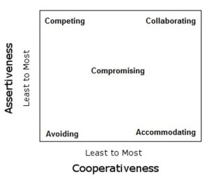
- The Thomas-Killman Conflict Mode Instrument depicts five methods for resolving conflict: competing, collaborating, compromising, avoiding, and accommodating. These methods of conflict resolution can be mapped to a matrix of values based on the method’s assertiveness and cooperativeness.
- Accommodating is the least assertive but the most cooperative of the conflict resolution methods.
- Competing is the most assertive and the least cooperative of the five conflict resolution methods.
- Avoiding is the least assertive and the least cooperative of the five conflict resolution methods.
- Collaborating is the most assertive and the most cooperative of the five conflict resolution methods.
- Process Decision Program Charts (PDPCs) are used to chart a course of events. PDPC map out as many contingencies and plans are made for each one.. PDPCs are appropriate for new, unique, and complex problems. Problems with multiple, complex steps are well suited for PDPCs.
- Interrelation Diagraphs (IDs) are appropriate for complex problems where the exact relationship between the problem’s elements is not easily identifiable. IDs are not used to plan for contingencies
- Affinity Diagrams organize and present large amounts of data by grouping like data into logical categories as perceived by the users. Affinity Diagrams are not used to plan for contingencies.
- Matrix Diagrams are used to show a relationship between two items. These diagrams consist of a table of rows and columns. Each row and column contains an item and the intersection of these rows and columns contain data on their relationship. Matrix diagrams are not used to plan for contingencies.
- Models
- IDOV – Identify, Design, Optimize, and Validate is a Design for Six Sigma (DFSS) methodology used to achieve Six Sigma levels of quality in new products and processes.
- CQFA – Cost, quality, features, and availability model describe 4 factors that make up value in the eyes of the customer. A business process needs to excel in at least one of these categories while meeting satisfactory levels in the others.
- SIPOC – A Supplier, Input, Process, Output, Customer (SIPOC) diagram models a closed loop business system for process management, improvement, and design. When suppliers in the SIPOC model are also customers, communication is channeled through internal company processes. Each supplier/customer supplies a different input and expects a different output from the process. In the case of employees and managers. the input is commitment and leadership respectively and the expected output is pay and career growth. While employees do expect career growth as an output of the process, stakeholders expect profit and company growth. The community expects tax revenues from the process while customers expect goods and services. Suppliers expect additional orders from the process while society expects an increase in quality of life.
- DMADV – Define, Measure, Analyze, Design, and Verify (DMADV) is a Design for Six Sigma (DFSS) methodology used to achieve Six Sigma levels of quality in new products and processes.
- A failure mode and effects analysis (FMEA)
| Issue |
Prob-ability |
Sev-erity |
Effect-iveness |
| A |
4 |
4 |
7 |
| B |
9 |
5 |
1 |
| C |
6 |
4 |
2 |
| D |
5 |
4 |
7 |
The Risk Priority Number (RPN) is calculated by multiplying Probability * Severity * Effectiveness. The highest number should be addressed first. Case D has the highest Risk Priority Number (RPN) (A 112, B 45, C 48, D 140) and should be addressed first (Skillsoft, 2010).
- A Failure Mode Effects and Criticality Analysis (FMECA) is a detailed analysis of a system. FMECAs examine the system down to the component level and classify items into three categories; failure mode, effect of the failure, and probability of the failure’s occurrence. After an item is categorized, it is assigned a criticality value based on how the failure will affect the system as a whole. Higher criticality values indicate a serious effect on the system.
- The following table shows six lots of items from a production run of 100 items and the number of defects found in each lot.
| Defects |
0 |
1 |
2 |
3 |
4 |
5 |
| Units |
60 |
18 |
10 |
6 |
4 |
2 |
Given that there are eight opportunities for defects in the process. what is the defects per million opportunities (DPMO) of this process? To calculate DPMO, you must first calculate the defect per unit (DPU). DPU is calculated by summing the products of the defects and the units per lot, and then dividing the result by 100.
DPU = [0(60) + 1(18) + 2(10) + 3(6) + 4(4) + 5(2)] / 100
DPU= [0+18+20+18+16+10] /100
DPU = 82 / 100
DPU = 0.82
Next, we must determine the number of defects per opportunity (DPO). This is calculated by dividing the DPU by the number of opportunities for defects, in this case eight.
DPO = 0.82 / 8
DPO = 0.1025
Finally, DPMO is found by multiplying the DPO by a million (10*6).
DPMO = 0.1025 * 10*6
DPMO = 102,500
- Calculate Total Defects per Unit (TDPU)
|
Step 1 |
Step 2 |
Step 3 |
Step 4 |
Step 5 |
Step 6 |
| Yield |
98% |
99% |
96% |
97% |
95% |
98% |
Rolled Throughput Yield (RTY) is a cumulative calculation of yield over multiple process steps. RTY is often used as a baseline metric for improvement projects. RTY is calculated by multiplying the yield from each step of the process.
RTY = .98 * .99 *.96 * .97 *.95 * .98
= .8411
TDPU can be calculated by finding the negative natural logarithm of Rolled Throughput Yield (RTY).
TDPU = -ln(0.8411)
= 0.1730
- Business Process Management (BPM) improves quality through the quality management approach. A manufacturing process will naturally flow across multiple vertical functions and pass through various horizontal business levels in the company. Traditionally, each vertical unit would be responsible only for their portion of the process. This means that managing the process across these transitions is difficult, as no one is responsible for the process as a whole. Confusion and defects are often the result of differences in the various units and levels in the company. BPM addresses this issue by using a project management approach. Project management ensures that someone is responsible for the process as a whole. Since one person has a good overall view of how the product will progress through the company, they are better able to make decisions relating to local functions that will affect the overall business outcome. Business process management involves collecting customer data at three levels: the business level, the operations level, and the process level. Customers who influence the operations level are those who purchase the company’s product or those employees who manage production operations. The operations level is concerned with gathering performance data and data relating to operational efficiency. Data is typically gathered at the operations level daily or weekly and is analyzed using Six Sigma methods and lean manufacturing principles. A supplier of raw material for the company’s product would influence the company at the process level. A member of the company’s top management, and a shareholder owning stock in the company would
influence the company at the business level.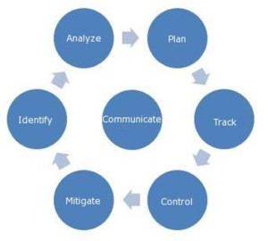
- Barbara Frank et al. refer to risk analysis and management as a continuous process in their Certified Software Quality Engineer (CSQE) Primer. They show this as a continuous six-step process circling a seventh step. Communicate. as a transition to each other step. When diagramed, this model appears as presented in the following exhibit.
- Teams
- Cross functional teams are normally made up of individuals from various departments within an organization. Cross functional teams are best suited for handling issues related to an organization’s policies, practices, and operations.
- Project teams are best suited to work on projects that are delivering new products or services.
- The “Quality teams” option is incorrect. Quality teams are created to work on improving performance or quality.
- Six Sigma teams work on important customer projects or distinct processes.
|
|
- 6s Measure
 Control Chart – shows the change in scores for an attribute over time. To help distinguish normal statistical variation from variation that is caused by specific events or unusual deviation, you add control limits to your chart. Control limits (LCL and UCL) are calculated using a formula set by a statistician. A control chart is a line graph that plots variable data, resulting in a dynamic visual representation of a process’s behavior. Control Chart – shows the change in scores for an attribute over time. To help distinguish normal statistical variation from variation that is caused by specific events or unusual deviation, you add control limits to your chart. Control limits (LCL and UCL) are calculated using a formula set by a statistician. A control chart is a line graph that plots variable data, resulting in a dynamic visual representation of a process’s behavior.
- Histogram is a graph that displays frequency of data within a given bar. The histogram shows a static picture of process behavior.
- Normal distribution is a bell-shaped distribution in which any special cause of process variation is removed from the data plotted.
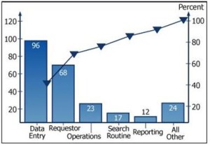
- Pareto Chart is reliable way to identify the vital sources of error that create a disproportionate number of problems in a project, kind of a type of histogram. The causes of error are listed in descending order on the x-axis. Pareto analysis is based on the principle that 20% of problems cause 80% of the occurrences. A Pareto diagram is a bar chart of each of the problem categories mapped to the number of problem occurrences. Problem occurrences are ordered from highest to lowest with one exception. Miscellaneous occurrences, regardless of number, are always displayed at the end of a Pareto diagram. Pareto diagrams have a second vertical axis included on the right side of the chart labeled as Percentage. The values on that axis go from 0 to 100. A cumulative line for the bar’s percentages is plotted using the Percentage axis and the plot rises from left to right. Pareto analysis is often done to achieve a new perspective on a problem, to prioritize problem occurrences, to compare changes in data between periods of time, or to create a cumulative line (Skillsoft, 2010). The Pareto principle (also known as the 80-20 rule, the law of the vital few, and the principle of factor sparsity) states that, for many events, roughly 80% of the effects come from 20% of the causes. Business management thinker Joseph M. Juran suggested the principle and named it after Italian economist Vilfredo Pareto, who observed in 1906 that 80% of the land in Italy was owned by 20% of the population (Wikipedia, 2010).
- Measles charts are a locational form of a check sheet. they are used to display the location of a defect by marking it on a schematic of the product. Measles charts are also used to map injury data on a human shaped schematic.
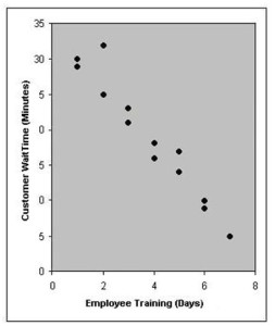
- Scatter Diagram – tells you about the nature of the relationship between the variables associated with the variation you are investigating. The casual variable represents the x-axis and the result variable represents the Y-axis. There is a best fit line but there are no LCL and UCL. Scatter diagrams are used to reflect the hypothesis about a credible variable that may be affecting another. The scatter diagram in the exhibit depicts a correlation coefficient as -1.0. A correlation coefficient of-1.0 is depicted by a high customer wait time at the beginning of the employee training and decreases at a constant rate as the number of employee training days increases.
- Fishbone Diagram – or cause and effect diagrams is a simple graphic display that shows all the possible causes of a problem. The problem becomes the head of the fishbone. Next you establish the major categories that cause the problem through brainstorming, then investigate 2 or 3 of them. The cause-and-effect diagram is a tool that can be used to break down a problem into manageable pieces. The cause-and-effect diagram is also known as a fishbone diagram or Ishikawa diagram. The problem statement is represented at the head of the fish and the causes are represented as the bones.
- Analytical studies use inferential statistics to predict what a process is capable of doing. Six Sigma relies on inferential statistics to help explain why a variation is occurring, whether it can be attributed to a given cause, and how reliable the inference itself may be. Sampling distributions, confidence intervals, and hypothesis testing are commonly used as the bases for making inferences about a population.
- Enumerative studies use descriptive statistics to describe a current process. Descriptive statistics tell the nature of what is happening in a given process using observations about the location, spread, and shape of data distribution around a central tendency.
- F Distribution tests – Named for its inventor Ronald Fisher, the F Distribution tests the null hypothesis that the variance of all population means under study are equal. The F Distribution is similar to the Student’s t Test, except that it examines the variance of multiple sample means, rather than the means themselves.
- The Student’s t Test or Students t Distribution was developed in 1908 by William S. Gosset, a chemist for the Guinness brewery. The t Test formula finds the difference between sample mean and population mean. and divides this by the standard error. Standard error is the standard deviation divided by the square root of the sample mean; dividing by standard error accounts for the variability between samples.
- Analysis of variance (ANOVA) is also commonly referred to as the f test or the f ratio. Instead of using the normal distributions z or t statistics, it uses a statistic based on the f distribution. ANOVA compares the variance between components (the variance around the individual means) to the variance within the components. The variance within the components is the estimate of the variance you can expect from random error.
- The term “muda” was introduced by Toyota’s Chief Engineer, Taiichi Ohno, and was used to describe waste that occurs in business. Being able to identify waste types in your company is the first step in eliminating non-value added activities from your production cycle, and ultimately increasing productivity and profitability.
- Inventory is one of the seven categories of muda (waste) widely used in industry. Inventory is considered waste as it does not add value to a product or to the consumer and requires extra space, transportation, and materials. Examples of inventory include parts. raw material, semi-finished goods (also known as work-in-progress), supplies, and finished goods.
- Overproduction muda occurs when more product is created than is required by the consumer.
- Repair, or reject muda occurs when a defective part must be repaired or reworked. The process of repairing or reworking the product adds no value to the consumer of the final product.
- Motion muda occurs when a process requires inefficient use of human motion. Examples of motion muda include excessive walking, heavy lifting, bending awkwardly, overreaching, and repetitive motion.
| Issue ID |
Length
(mm) |
| A |
2.01 |
| B |
2.05 |
| C |
1.98 |
| D |
2.04 |
| E |
2.03 |
- To calculate the standard deviation. we must first calculate the mean of the values, followed by the variance. Once the variance is calculated, standard deviation is found by taking the square root. To calculate the mean, add all the values together and divide by the number of values present.
Mean = (2.01 + 2.05 + 1.98 + 2.04 + 2.03) / 5
= 10.11 / 5
= 2.022
To calculate variance (V), find the sum of the squares of the differences between the mean and the given value, and divide it by the number of values minus one. Note that we divide by the number of values minus one because sample size is below 30 (to remove potential bias from the small sample size).
V = [(2.01 – 2.022)^2 + (2.05 – 2.022)^2 + (1.98 – 2.022) ^2 + (2.04 – 2.022)^2 + (2.03 – 2.022)^2] / (5 – 1)
= 0.00308 / 4
= 0.00077
Finally, to calculate standard deviation (StdDev). take the square root (SQRT) of the variance.
StdDev = SQRT (V)
= SQRT(0.00077)
= 0.0277
- A sample of 20 plastic bags is randomly taken from a continuous process where the population is 1000 plastic bags. Past studies have demonstrated that 15% of the bags contain defects. What is the probability of finding two defective bags? The binomial distribution is used to model discrete data in the situation with two possible outcomes. The two possible outcomes are defective plastic bags and non-defective bags. The binomial distribution is generally applied in situations where the sample size is less than 10% of the population. Therefore, we can use the binomial probability distribution function to determine the probability of finding two defective bags within the sample. The binomial probability distribution function is stated as follows:
P(r) = n!/(r! * (n-r)!) * p^r*(1 – p)^(n-r)
n = Size of the given sample = 20
r = Occurrences of the number of defective units = 2
p = Probability of defective units = 0.15
P(2) = 20!/(2! * (20-2)!) * (0.15)^2*(1 – 0.15)^(20 – 2)
P(2) = 2432902008176640000 / 12804747411456000 * 0.0225 * 0.05365
P(2) = 190 * 0.0225 * 0.05365
P(2) = 0.22935 = 22.94%
- The mode of a dataset is the most frequently recurring value.
- Mean is calculated by finding the average of all data in the set. It is calculated by
finding the sum of the dataset’s values and then dividing by the number of values in the set.
- The median of a set of data is the middle value when the data is sorted in an
ascending or descending order.
- Range is a measure of dispersion. Range is calculated by finding the difference between the highest and lowest values in the dataset.
- Variable Data is measured and continuous, it includes measurements of length, volume, time, or area (e.g. Depth of cut.
- Attribute Data is discrete and is often referred to as counted data, as it may only consists of integers. e.g. welds per unit, scrapped parts, number of scratches
- Statistic is defined as a data value from a sample that is in the form of a number, which then can be used to make an inference about a population. e.g. standard deviation or variance of a sample.

- Cp and Cpk are process capability indices. They evaluate short-term process capability. Cp does not take process centering into account. Cpk does take process centering into account.
- Pp is a process performance index that indicates a process’s ability to produce products within specifications over a long period of time. Pp does not take process centering into account. Pp is calculated using the following formula:
Pp = (USL – LSL) / 6 sigma
- Ppk is an indicator of long-term process performance, it takes centering into account. The process performance index (Ppk) is an actual measure of a process’s performance. To calculate Ppk, the following formula should be used:
Ppk = minimum ( (USL – X-bar) / 3 sigma, (X-bar – LSL) / 3 sigma )
- The actual observed sigma is calculated using the following formula:
Sigma = Square root: ( Sum (X – X—bar)^2 / (n – 1) )
- This formula is an estimation of sigma used for process capability indices (Cp and Cpk).
Estimated Sigma = R-bar / d2
- Quantifying Measurement Errors Methodologies
- The range method is the simplest of the three methods for quantifying measurement errors. The range method does not separate reproducibility and repeatability in its quantification.
- The Analysis of Variance (ANOVA) method separates repeatability, reproducibility, part variance. and variability in the interactions between appraisers and the parts being measured.
- The Average and Range method separates repeatability, reproducibility, and part variance.
- Sampling Techniques
- A lot of parts produced from different sources and produced using different machines or processes is said to be a stratified group. To properly take differences in the source parts into account, stratified sampling must be performed. Stratified sampling randomly selects samples from each distinct group of parts. For example, parts from each of the manufacturing plants would be considered a separate group. This allows the number of samples from each group to be changed based on the proportion of parts being used from that group.
- In multiple or sequential sampling, a lot of parts is accepted or rejected based on the results of analyzing samples. After each sample is examined, either a decision to accept or reject the lot is made or another sample is taken. With multiple sampling, a decision must be made before a specified maximum number of samples are examined. With sequential sampling, sampling can theoretically go on indefinitely; however, sampling usually stops once the number of inspections has exceeded three times the sample size of the sample plan.
- Random sampling randomly chooses a sample from an entire lot. The lot is then accepted or rejected based on this sample. Truly random sampling is difficult to achieve since you must ensure that each item in a lot has an equal chance of being selected as the sample unit.
- Having an operator make similar measurements close to the same time is known as precision. With precision, the data values are located within close proximity to one another but are located a distance away from the true value that contains no bias.
- Calibration refers to the comparison of a measurement instrument, or system of unverified accuracy, to a measurement instrument, or system of known accuracy, to detect variation from the required performance specification.
- The term nominal in Six Sigma refers to a measurement scale. The nominal scale is made up of data based on categories or names. There is no ordering involved in the nominal scale.
- Accuracy refers to the variance between the actual value that contains no bias and the average value among the number of measurements.
- 6s Analyze
- The Welch-Satterthwaite equation is used to determine the degrees of freedom for the 2 mean unequal variance t test.
- One-Way Analysis of Variance (ANOVA) test there are 3 different degrees of freedom:
- Total Degrees of Freedom (Total DF) – Total number of error points minus 1
- Treatment Degrees of Freedom (TDF) – Number of treatments minus 1
- Error Degrees of Freedom (EDF) – Total DF minus the TDF
- In a one-way analysis of variances (ANOVA), the treatment sum of squares (SST) must be calculated to find the total sum of squares. To calculate SST, find the sum of the squared deviations of each treatment average from the grand average.
- Corrected sum of Squares – By finding the difference between the crude sum of squares and the correction factor
- Error degrees of freedom – By finding the difference between the total degrees of freedom and the treatment degrees of freedom
- Experimental Error Sum of Squares (SSE) – By finding the sum of the squared deviations of each observation within a treatment from the treatment average
- F-Test is used to test if two sample variances are equal. The precisions of measuring devices are often compared to each other by testing the variances in their measurements. This inference test is used to test the variances of two samples that are equal. To facilitate this test, the variances of two samples are compared for equality. This is done using the F test paired-comparison test.
- Paired Test is used to detect differences in two population means. Data is collected in pairs and a difference is calculated for each sample
- T Test – The “2 mean unequal variance t test” and “2 mean equal variance t test” are used to test the difference between two sample means when the variances of the samples are unknown.
- Z-Test is used to compare a single population’s mean with a fixed value
- 3 Methods for quantifying measurement errors
- ANOVA separates repeatability, reproducibility, part variance, and variability in the interactions between appraisers and the parts being measured. ANOVA is the is the most accurate for quantifying measurement errors.
- Range Method is the simplest of the 3 methods for quantifying measurement errors and does not separate reproducibility and repeatability in its quantification.
- Percent Agreement Method is a percentage representing how close a measurement is to a reference or actual value and is NOT a method for quantifying measurement errors.
- Average and Range Method separate repeatability, reproducibility and part variance; however, it is not as accurate as ANOVA.
- Nominal in Six Sigma refers to a measurement scale. The nominal scale is made of data based on categories or names. There is no ordering involved in the nominal scale.
- Z test hypothesis test, you compare a test statistic to a critical value. The critical value is based on a confidence interval and is taken from the a standard Z table. You can denote the test as a two-tail, right one-tail, or left one-tail with the comparison operator specified in the alternate hypothesis. If the sign in the alternate hypothesis is not equal (!=), the test is a two-tailed test. If the greater than sign (>) is used for an alternate hypothesis, it is a right one-tailed test. A left one-tailed test is indicated by a less than sign (<) in the alternate hypothesis (Skillsoft, 2010).
- Equation for Sample Size involving normally distributed data:
- Z = 1.96
- Sigma = 36,000
- E = 12,000
- n = Z^2*sigma^2/E^2
| Dog |
Drugs
Found |
Drugs
Not Found |
| 1 |
17 |
3 |
| 2 |
18 |
2 |
| 3 |
16 |
4 |
| 4 |
20 |
0 |
- Four dogs are being evaluated for use on a drug detection team. To test the dogs, 20 packages of drugs are hidden throughout a lot of luggage. Determine whether there is a significant difference between the dog’s ability. You decide to use the chi-squared test with a confidence interval of 95%, what is the critical value (X-Squared)? The null hypothesis is that there is no difference between the dogs’ ability to find drugs (H0: p1 = p2 = p3 = p4). To find the critical value, when comparing observed and expected frequencies of test outcomes for attribute data, we need two pieces of information: confidence interval and degrees of freedom. In this example, the confidence interval is 95% (alpha = 0.05) in the one tail, right side of the distribution. The degrees of freedom (DF) is found using the following formula:
DF = (number of rows – 1) * (number of columns – 1) = 3
From a chi-squared distribution chart, the critical value for a right-sided, one-tail test with DF of 3 at a 95% (0.05) confidence level is 7.81.
- Variation Types
- Cyclical variation refers to a variation from piece to piece or unit to unit. It can also be a variation from one operator to another or from machine to machine. When the same functions performed by different machines produce different results, cyclical variation can be indicated.
- Temporal variation is a time-related variation. Patterns of charting data over time indicate that time is a factor, and the patterns can help point to causes by identifying when the variation occurs.
- Ordinal variation is a measurement scale in which data is presented in a particular order. The differences among the data values cannot be assigned any meaning or the differences have no real significance.
- Positional variation is variation that can occur within a piece, batch unit, part, or lot.
- A regression analysis has been performed on the study for Customer Complaints versus Time for Training. The p value is calculated to be 0.04. This indicates that the Time for Training is a statistically significant factor contributing to the customer complaints.
- A p value of 0.04 indicates time for training is a statistically significant factor contributing to the customer complaints. In statistics. “significant” means probably true or not due to chance. When testing statistical significance, a calculation is carried out based on sample information. In regression analysis, the slope of the line (known as beta) relates to the coefficient, which is Time for Training in this scenario. The p-value of 0.04 suggests that the Time for Training coefficient is a statistically significant factor.
- To have a highly significant statistical factor, the p value would need to be less than or equal to 1%. The p value in this scenario is 0.04 or 4%.
- To satisfy the condition of not being a significant statistical factor, the p value would need to be greater than 5%. The p value in this scenario is 0.04 or 4%.
- The p-value is used to denote statistical significance, not practical significance. There are two categories of significance: statistical significance and practical significance. The term practical significance is used to describe the usefulness or importance of research.
- Type I error – When performing a hypothesis test, rejecting the null hypothesis when it is true is considered a Type I error. The symbol for alpha is used to denote the probability of making this type of error. By definition, the null hypothesis can only be rejected or fail to be rejected. It cannot be accepted.
- Type II error -When performing a hypothesis test, not rejecting the null hypothesis when it is false is considered a Type II error. The symbol for beta denotes the probability of making a Type II error.
|
|
- 6s Improve and Control
- Control Plans are developed to ensure changes made to a process remain effective.
- Failure Modes and Effects Analysis (FMEA) may assist you in finding the next target for improvement.
- u Charts – Tracks the average number of defects with variable sample size
- c Chart tracks the where the sample size is fixed, both u & c charts assume a Poisson distribution for defects.
- p Charts tracks information relating to the number of defective products, not the number of defects. The p chart tracks percent defective with a variable sample size.
- np Chart simply tracks the number of defective products in a fixed sample size. Both the p and np charts assume a binomial distribution of defectives. An np chart is used for attribute data. It is especially well suited for when you need to evaluate a count of defective or non-conforming items produced by a process. The np chart data must be unit counted and the subgroup size must remain constant.
- X-bar – R charts, MX-bar – MR charts, and median charts are only appropriate for variable data.
- Experiments:
- Replication – Performing an experimental run multiple times by completely breaking down the setup and set points (settings) between runs is known as replication Replication is performed to reduce the effects of variations that are part of the process.
- Parallel experiments are experiments that are run simultaneously. Parallel experiments are contrary to sequential experiments where one experiment is performed at a time after the previous experiment.
- Repetition occurs when performing an experimental run multiple times without breaking down the setup and set points between runs. Unlike replication, repetition does not reduce the effects of variations that are part of the process.
- Sequential experiments occur by having one experiment performed at a time after the previous experiment. This is the opposite of parallel experiments.
- Levels refer to the various settings being tested in the experiment.
- The factor is the independent variable that is not affected by another variable.
- The main effect is determined by measuring the mean change of an output factor during the process of changing levels. For example, if changing the weight from 2 grams to 6 grams does not change the length of the material, then the main effect is no change.
- Residuals are the differences between observed values and the corresponding values predicted by a model. For example, once you have come up with a line that fits the data in a regression analysis, you can determine how well the line tits by looking at the residuals.
|
|
- References
- How Stuff Works (2010). Retrieved from http://money.howstuffworks.com/six-sigma7.htm
- Innovating To Win (2010). Retrieved from http://www.innovatingtowin.com/innovating_to_win/2007/06/six_sigma_and_i.html
- MiC Quality – Six Sigma Glossary (2010). Retrieved from http://www.micquality.com/six_sigma_glossary/takt_time.htm
- Engineering Statistics Handbook (2010). Retrieved from the web,What are Attributes Control Charts?http://www.itl.nist.gov/div898/handbook/pmc/section3/pmc33.htm
|
|
This page was last updated on March 27, 2021 |